Artificial Intelligence: Practical A/B testing in Microsoft Fabric

Experimentation is the only way to know whether a model improves real decisions; without a well‑designed A/B test you are merely guessing.

Why do A/B testing for AI models?

In a business context, an AI model is not just a technical artefact — it is a decision component that impacts revenue, costs and user experience. A new model that promises higher accuracy can in practice alter user behaviour, increase operational costs or introduce undesirable side effects. A/B tests bring the necessary evidence: with an appropriate experimental design you can evaluate the causal effect of the model on real business metrics and avoid decisions based only on offline metrics (ROC, AUC, loss).

Offline metrics tell you how well a model predicts a label on labeled data; A/B tests tell you the economic impact of that prediction when integrated into an application. For example, a fraud detection model with improved AUC can also increase false positives in production and, as a consequence, block legitimate wallets — translating into lost revenue and customer friction. A well‑planned A/B test quantifies that trade‑off in terms of churn, revenue, cost per acquisition (CPA) or fraud reduction.

For organizations using Microsoft Fabric, integrating A/B tests into pipelines brings operational advantages: version control, persistence of assignments, centralized telemetry and the ability to automate analyses in production. Instead of relying on ad‑hoc scripts, you can create reproducible flows that record who was exposed to which version, when and with which features — reducing the risk of regression when deploying new models.

Practical architecture in Microsoft Fabric

A pragmatic architecture for A/B testing in Fabric combines familiar components: Lakehouse (Delta) for raw data, metadata and scoring results; Spark Notebooks or Jobs for feature preparation and batch scoring; pipelines for orchestration; and Power BI for monitoring experimental results. The central idea is to treat the experiment as a first‑class citizen on the platform.

Typical components and responsibilities:

• OneLake / Delta Lake: storage for events, experimental assignments and scoring results. Structure tables by experiment_id and by date for easy partitioning and cleanup (for example: experimental_assignments(partition: experiment_id, dt), experiment_results(partition: experiment_id, dt)).
• Spark Jobs / Notebooks: feature preparation, deterministic hashing/assignment and batch scoring for large volumes. Use scheduled tasks for re‑scoring when there is retraining or new features.
• Orchestration pipelines (Data Factory/Sync-like): sequence of steps with checkpoints — ingestion → assignment → scoring → metric aggregation → dashboard publication.
• Streaming (when necessary): event ingestion in near real‑time for click/conversion metrics using connectors; consolidate in micro‑batches to avoid excessive latencies.
• Power BI / Dashboards: reports with temporal evolution, group comparisons and integrated alerting with Azure Monitor/Teams for automatic rollback.

A typical flow implemented in Fabric:

1. Ingestion of events (application telemetry, transactions) into the Lakehouse.
2. Computation of the experimental unit (user/account/session) and execution of the deterministic assignment function to obtain the group (A/B) — persisting the assignment with timestamp and experiment version.
3. Batch or streaming scoring that reads the assignments table and applies the appropriate model version, writing results to an experiment_results table.
4. Consolidation of business events and technical telemetry to compute aggregated metrics by group and time window.
5. Publication of Power BI dashboards with automatic refreshes and alerts configured for critical thresholds.

In the Lakehouse design, include metadata columns: experiment_id, experiment_version, model_version, assignment_hash, assignment_ts, feature_hash. Optimize with Z‑ORDER by id_utilizador to accelerate joins between assignments and events. Retain assignment data for audit (at least 90 days or per regulatory requirements) and store model artefacts (binary, metadata) in the catalogue with a reference in the experiments table.

Experiment design and key metrics

Experimental design is where most projects fail — not for lack of technology, but for lack of rigor. Start by documenting the unit of randomization, primary hypothesis, secondary metrics, eligibility criteria, proposed duration and stopping rules. Without this, you risk post‑hoc analysis and falling into multiple comparison bias.

Unit of randomization: choose between user, account or session. The user unit is the most conservative (controls learning and behaviour over time) but requires larger samples; session gives faster signals but increases risk of contamination.

Typical metrics and how to operationalize them:

• Conversion rate (primary) — number of conversions / number of eligible visits.
• Average order value (AOV) — sum of transacted value / number of orders.
• Revenue per exposed user — combination of conversion rate and AOV, useful for direct comparisons per 1000 exposed users.
• Technical metrics — average latency, error rate, fallback rate (when the system falls back to the previous model).
• Safety metrics — false positives/negatives in fraud, impact on churn, user trust indicators.

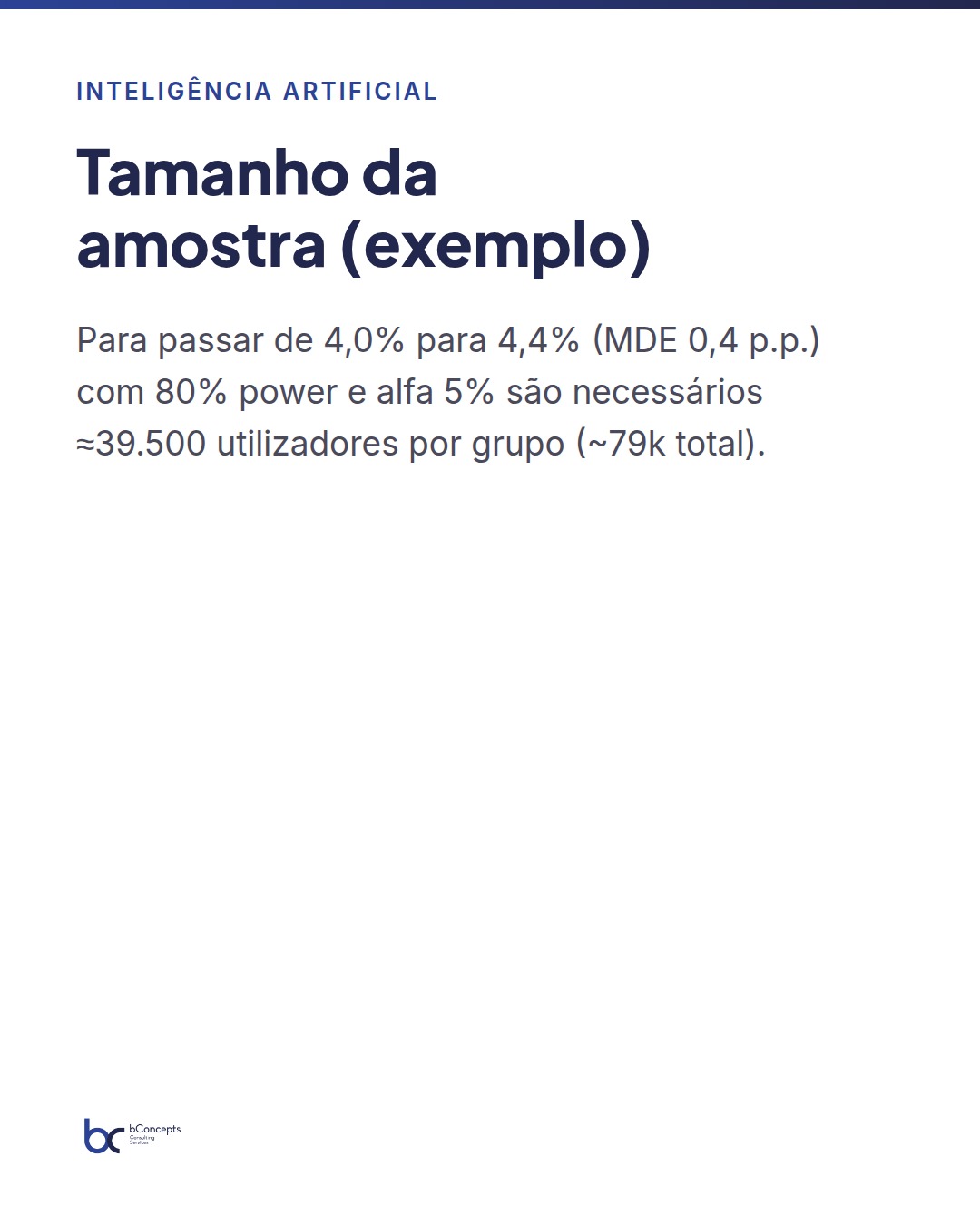
Sample size: calculate based on the baseline and the minimum detectable effect (MDE). Practical example: if the current conversion rate is 4.0% and you want to detect an absolute increase of 0.4 p.p. (i.e., to 4.4% — a relative gain of 10%), with 80% power and 5% alpha, the approximate calculation using the two‑proportion formula yields about 39,500 users per group (≈79k total). In other words, if you are randomizing by session instead of user, count sessions; if by user, count unique exposed users.

Also document stopping rules: for example, do not analyze before a minimum of 14 days and a minimum N per group; in sequential analysis use corrections (alpha spending) or a Bayesian framework with pre‑specified probability thresholds to reduce the risk of premature stops.

Step‑by‑step implementation

1) Identify experimental unit and records: decide whether the unit is the user (more conservative) or the session (more responsive). For retail and offer scoring scenarios, the account/customer unit is often the correct choice to prevent the same user receiving different versions within the same purchase period.

2) Implement deterministic assignment: generate a hash or HMAC function (e.g.: HMAC‑SHA256(id_cliente ∥ experiment_id ∥ salt)) and convert the hash to an integer that maps to percentile buckets. Practical example: bucket = int(hex_digest[:8], 16) % 10000 → if bucket < 5000 then group A, else group B; this ensures reproducibility even if the service is restarted. Persist this assignment in a Lakehouse table (for example experimental_assignments) with columns: id_cliente (string), experiment_id (string), grupo (char), assigned_at (timestamp), model_version (string), salt_version (string).

3) Scoring pipeline: create a Spark Job that reads experimental_assignments and applies the corresponding model. Structure the experiment_results table with columns: id_cliente, experiment_id, model_version, score, action_recommended, scored_at. Version model artefacts (model_v1, model_v2) and store the feature_hash to ensure you can reproduce exact scoring in the future.

4) Telemetry and business metrics: instrument the application to emit conversion/action events to an events table (event_type, id_cliente, value, ts). Consolidate these sources with scoring results to compute aggregated metrics by group and time window using scheduled jobs (for example, hourly aggregations for near real‑time dashboards).

5) Dashboards and analyses: build Power BI reports that show daily evolution of metrics by group, uplift estimates (absolute and relative differences), confidence intervals and segmentation tables. For large experiments configure refresh cadence hourly or daily depending on volume — for experiments with tens of thousands of users, daily reporting is the most stable to avoid noise.

Mini practical case: omnichannel retail

In an omnichannel retail company with 80 analytics team members and 1.2 million active customers, the bConcepts team implemented an A/B test for a new recommendation model that prioritizes margins instead of mere click probability. Hypothesis: increase average order value (AOV) without reducing conversion rate.

Key experiment parameters:

• Unit: customer (persistent for 30 days).
• Eligible population: 400,000 customers with activity > 3 purchases in the last year.
• Allocation: 50% control (current model), 50% treatment (new model).
• Planned duration: 28 days.

Results after 28 days (consolidated data):

• Conversion rate: 4.05% (control) vs 3.98% (treatment) — difference not statistically significant (p=0.18). With 200k customers in each group, estimated conversions were 8,100 vs 7,960.
• Average order value (AOV) among conversions: €58.20 (control) vs €63.10 (treatment) — absolute uplift €4.90, relative +8.4%, p<0.01.
• Revenue per 1000 exposed users: €2,358 (control) vs €2,520 (treatment) — uplift €162 per 1000 users.

Interpretation and decision: despite a small reduction in conversion rate, the AOV increase compensated and produced a material revenue gain. Scaling this, if the model is applied to 30% of the 1.2M active customers (360k), the expected uplift per 1000 users translates to ~€58k additional per month (360 × €162). The decision was a gradual rollout to 30% of traffic with close monitoring of conversion and impact on critical segments such as new customers and VIP customers.

Without controlled tests you are optimizing for offline metrics; with controlled tests you are optimizing for real business impact.

Monitoring, statistical analysis and rollout

During the experiment monitor primary metrics, secondary metrics and technical metrics (latency, errors, fallback rate). We recommend dashboards with three views: global view (KPIs by group), alerting (configurable thresholds) and diagnostics (segmentations and cohort evolutions).

For statistical analysis, compute point differences with confidence intervals. Bootstrap is particularly useful when distributions are skewed (for example AOV with a long tail). Practical approaches:

• Classical frequentist analysis for the primary hypothesis with p‑values and CIs — good for pre‑specified binary decisions.
• Bayesian analysis for continuous updates of the probability of uplift — useful when you need a probabilistic interpretation (e.g.: 92% probability that the treatment increases revenue).
• Corrections for sequential testing: if you intend to look frequently at the data, use alpha spending methods (O'Brien‑Fleming, Pocock) or a Bayesian framework to avoid inflating the false positive rate.

Controlled rollout: do not promote immediately to 100% of users. Typical strategy: canary 10% → 30% → 60% → 100% with observation periods between steps (e.g.: minimum 7 days and minimum N per group). Configure automatic rollback if safety metrics exceed thresholds (e.g.: drop in conversion rate >0.5 p.p. or increase in average latency >200 ms). Integrate alerts with Teams/Slack and orchestration pipelines to execute rollback actions if necessary.

Risks, mitigation and operations

Common risks include group contamination (users exposed to multiple versions), external events that affect behavior (marketing campaigns, seasonality) and infrastructure problems. Practical mitigations:

• Persistent and idempotent assignments — never reassign a user during the experiment period.
• Log external events (promotions, campaigns) as covariates to control in the analysis or stratify samples.
• Infrastructure integration tests — automatic validation of latency and error rate before increasing traffic.

Operationally, define clear responsibilities: Experiment Owner (product/PO), Data Engineer (creation and closure of experiments), Statistical Analyst (validation and reporting) and Production Engineer (rollback/monitoring). Establish an experiments catalogue in the Lakehouse with metadata: experiment_id, objective, hypothesis, start/end, owner, model_version, salt_version, state (draft/running/closed) — this facilitates audits and reproducibility.

In summary

• Define unit, hypothesis and metrics before any code: a poorly defined experiment generates wrong decisions.
• Implement persistent assignment in the Lakehouse and explicit model versioning in the Fabric for auditability.
• Compute samples and stopping rules; use frequentist and/or Bayesian analyses according to operational needs.
• Automate scoring and metric harvesting with Spark Jobs and feed Power BI dashboards for continuous monitoring.
• Plan gradual rollout with rollback thresholds and clear team responsibilities.

Conclusion — next steps: start with a pilot using a low‑risk experiment (for example, differences in offer prioritization), document the entire process in the Lakehouse and build a monitoring dashboard that combines business metrics and technical telemetry. If you already use Microsoft Fabric, review how assignments and model versions are persisted: small improvements here greatly reduce the risk of regression. A pilot with 50k users per group may be sufficient to detect relevant economic changes in many contexts — and provides the operational experience to scale experimental governance across the organization.

Ready to turn promising models into measurable gains? What controlled experiment could your organization launch in the next 8 weeks?