Data Engineering: essential metrics for pipelines

“If you don’t measure, you don’t control — and if you don’t control, you don’t improve: instrumenting pipelines is as critical as building the data.”

Why make pipelines observable?

Moving from “it works” to “we know it works” is a cultural and technical leap that separates fragile data projects from reliable platforms. Pipelines that run without visibility hide losses — duplicate rows, drops in volume, schema drift, or delays that are only noticed when they impact critical reports or business applications. These issues used to surface as crises: spikes in calls to the data team outside working hours, urgent reprocessings and temporary manual reports to work around information gaps.

Observability is not just logging. It means measuring actionable indicators: how many rows arrived, how long it took, how many failures occurred, what the quality of the most sensitive columns is. Without these metrics, the data team lives in a reactive cycle where many engineering hours are spent searching for causes instead of preventing impacts. A pipeline with good telemetry is, in practice, an operational health sensor: it reduces the time between problem occurrence and resolution, enables automated reactions and contributes to sustainable SLAs.

Furthermore, well-implemented observability feeds architectural decisions. When we know that 80% of runs take less than X seconds, but 5% exceed 10× that latency due to unbalanced partitions, we have concrete data to invest in repartitioning, compaction or format changes (for example, Parquet columnar with statistics). Without metrics, these optimizations remain in the realm of intuition.

Essential metrics for Data Engineering pipelines

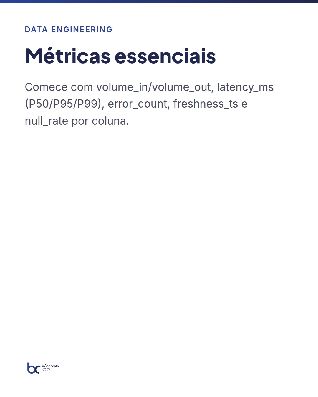
There are dozens of possible metrics, but start with a small pragmatic set that directly answers three questions: what arrived, how it arrived and when it arrived. I recommend inserting at least the following metrics in each pipeline run:

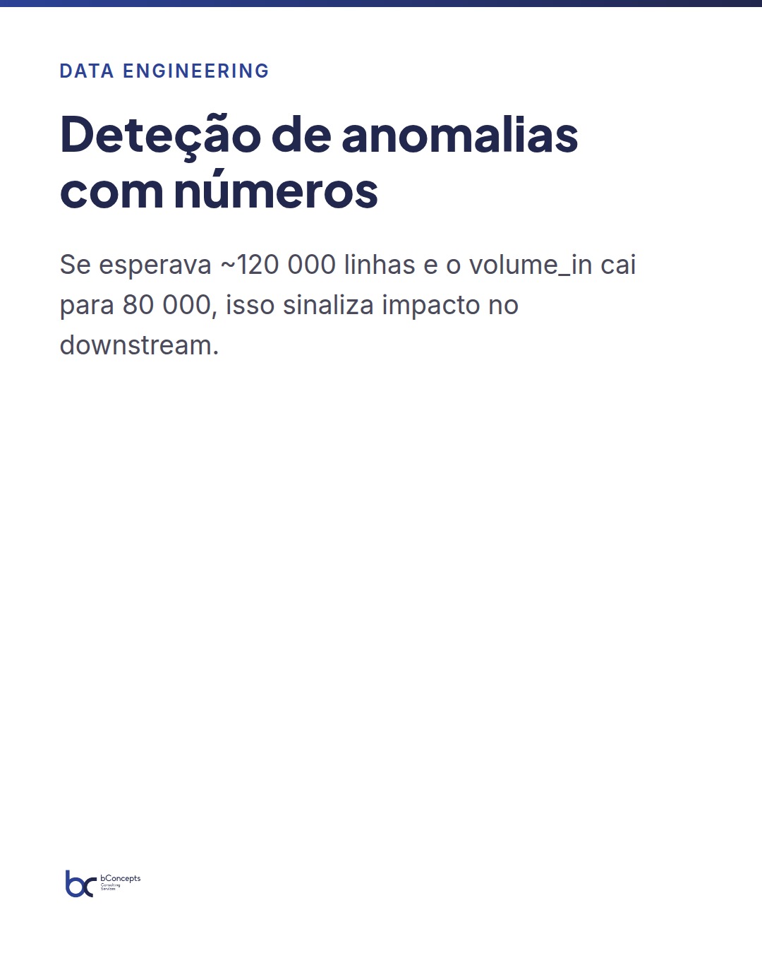
• volume_in / volume_out: number of rows read and written; measuring both allows identifying losses or duplications. For example, if a daily expected ingestion is ~120,000 rows and volume_in drops to 80,000, there is already an anomaly with clear downstream impact.
• latency_ms: total execution duration (start → end) and latencies per stage; also store percentiles (P50, P95, P99) to capture performance tails.
• error_count and error_rate: failures and percentage of records with errors; record error types (parsing, constraint, timeout) for prioritization.
• freshness_ts: timestamp of the most recent processed data; essential for near‑real time SLAs. Ex.: “freshness_ts is 45 minutes behind.”
• null_rate_por_coluna: percentage of null values in critical columns; measurement per column allows identifying quality degradation in sensitive fields (price, stock, customer_id).
• schema_signature: representative hash of the schema (columns+types) for quick drift detection; a simple SHA256 of the ordered text with names and types is enough to start.
• downstream_coverage: which reports or tables depend on that run (minimal lineage); this helps estimate the impact of a failure.

These metrics allow configuring simple rules: for example, alert if volume_in falls more than 30% versus the median of the last seven runs, or if null_rate in a critical column exceeds 5%. In high-volume environments, also define relative (percentage) and absolute (minimum number of rows) rules to avoid false positives when volumes are naturally small.

Measuring is not bureaucracy: it is reducing the time between failure and resolution from weeks to minutes.

How to instrument metrics in Microsoft Fabric and the Lakehouse

In the Microsoft Fabric context, the practical principle is simple: have your jobs emit structured telemetry to a central repository inside the Lakehouse and use Fabric pipelines to run validations and aggregations. You can leverage Spark Notebooks, Integration Pipelines and Jobs to insert metric records along the flow. Those records should be written in optimized formats (Parquet/Delta) for fast analytical reads.

A recurring pattern is as follows: each job (ingest, transform, aggregate) writes one telemetry row to a metrics table hosted in a Lakehouse dedicated to observability. That write is atomic with the run (i.e., written at the end of the run with commit), ensuring dashboards reflect the effective state of the runs. In distributed scenarios, include a checkpoint or completion mark that guarantees consistency across multiple steps.

More concretely:

1. at the start of the job, create a unique run_id (UUID) and record a 'start' event with metadata (source, load_parameter, expected_rows, shard_id); this eases correlations in logs and tracing failures by run_id;
2. during processing, emit intermediate metrics (e.g.: rows_read per stage, aggregated values of fields, exception counters by type) to identify slow steps or corrupted data;
3. at the close, write an 'end' event with volume_out, elapsed_ms, error_count, schema_signature and a sum of quality records; include a status field (success/partial_fail/fail) and a link to logs;
4. use an aggregation process (e.g. an hourly notebook) to calculate medians, percentiles and baselines for alerts and feed dashboards; keep a short retention window (30–90 days) for detailed metrics and a historical aggregated table for 1/7/30 day trends.

To cover communication failures between components, include retry attempts for telemetry writes and, in critical scenarios, persist metrics also to a queue (e.g.: staging area in ADLS in Parquet format) for eventual processing. A robust pattern is to write first to local/temporary files and only then atomically commit to the central table — this protects against losses in immediate network failures.

Metrics table design and data contracts

The metrics table schema should be simple and optimized for analytical queries and low-latency alerts. A practical example of columns:

run_id STRING, pipeline_id STRING, start_ts TIMESTAMP, end_ts TIMESTAMP, volume_in BIGINT, volume_out BIGINT, error_count INT, error_rate DOUBLE, freshness_ts TIMESTAMP, schema_signature STRING, null_rate JSON, tags JSON, status STRING, host STRING

I recommend partitioning by date (start_ts) and, when the run volume is large, by pipeline_id to reduce scans. Store null_rate and tags as JSON for flexibility — but document these fields in the data catalog (or in a README file) to ensure consumers know how to interpret the values. For example, null_rate may look like {"price": 0.02, "customer_id": 0.0}.

Besides the runs table, keep a thresholds and SLAs table (pipeline_id, metric_name, threshold_value, window_minutes, severity). This allows dynamic rules without changing code: a critical alert can be adjusted in production by simply updating a record in this table. Ex.: for the orders pipeline, a record could say: (orders_ingest, volume_in, 84000, 1440, high) meaning if the 24h average volume is below 84k rows, trigger a high severity alert.

Also consider maintaining a small schema registry with history of schema_signature and descriptions of changes to simplify rollbacks or drift management.

Alerts, SLAs and integration with Power BI

A good strategy is divided into three layers: detection, notification and reaction. For detection, apply rules over the metrics table (e.g.: rolling median of the last 7 runs). For notification, use mechanisms your organization already accepts — and in the Microsoft ecosystem this can include e‑mail via Logic Apps, Teams via webhook, or direct alerts in Power BI for key users.

In Power BI create a pipeline “health” dashboard: cards with last status, average times, 95th percentile latency and trend charts for volume_in. Visually configure thresholds with colors (green/yellow/red) and add bookmarks for drill‑downs by pipeline. Examples of practical rules:

• Alert if volume_in < 70% of the median of the last 14 runs (medium severity).
• Critical alert if error_rate > 2% and error_count > 100 in a run.
• Alert if freshness_ts is more than 30 minutes behind the SLA for near‑real time data.
• Alert if the P95 of latency_ms exceeds 5× the historical value, indicating a performance regression.

For 24/7 operations, integrate with the incident system (e.g. ServiceNow, Opsgenie). The goal is not to multiply alerts, but to ensure each alert has an owner and a clear playbook (how to reprocess, how to rollback, or how to communicate to the business). Define severity levels and expected response times (SLOs), and track an “error budget” to assess when structural interventions are needed instead of ad‑hoc fixes.

Mini practical case: online retail that reduced resolution time by 80%

In an online retailer with 120 employees, where the data team was 6 people, the nightly ingestion pipelines processed on average 41,095 orders/day (≈15M/year). Before instrumenting metrics, the organization detected irregularities through reports from BI teams or customers, with average time to detect a failure of 12 hours and average time to resolve of 18 hours — a total of 30 hours per incident. There was an expensive cycle: reprocessings during traffic peaks that increased compute and temporary storage costs.

Concrete steps they implemented:

1. definition of the 8 essential metrics per pipeline and telemetry templates (reduced variation between new/old pipelines);
2. implementation of atomic writes to the metrics table in the Lakehouse and redundancy in Parquet files in ADLS for cases of immediate write failure;
3. creation of Power BI dashboards with visual thresholds and alerts via Teams and e‑mail to owners;
4. simple playbooks: reprocess X hours, apply transformation patch, and communicate impacted parties; and 2‑hour training for all BI team members on how to interpret the dashboards.

In three months they observed the following measurable results:

• average detection dropped from 12h to 15 minutes;
• average resolution reduced from 18h to 6h (average total time per incident: 6.25h vs 30h);
• number of incidents impacting monthly reports decreased 60% (from 5 to 2 per month);
• operational costs of the data team associated with firefighting decreased by about 35% (estimate: 0.8 FTE of time freed for improvement projects).

In a conservative calculation: if an engineer costs €60,000/year (including charges), 0.8 FTE equals €48,000/year saved or reallocated to innovation. To these direct benefits add reduced compute spending due to fewer re‑executions in large windows (they estimated a 20% reduction in cluster costs during peak hours). More important was the qualitative gain: stakeholders trusted the SLAs more, reducing manual escalations and ad hoc work.

Operational best practices and light governance

Instrumentation alone does not solve — it needs processes. Define clear ownership: each pipeline has an operational owner and a documented playbook (how to restart, how to reprocess, rollback points). Establish short weekly review meetings for critical pipeline metrics and a quarterly threshold review process with business stakeholders. This ensures thresholds reflect business reality and not just old technical values.

Avoid metric overload. Start with 5–8 essential signals per pipeline and evolve iteratively. Document the meaning of each metric and, whenever possible, automate metric creation from templates for new pipelines — this reduces friction and ensures consistency. For governance, keep a small set of policies: retention of detailed metrics (30–90 days), anonymization of sensitive fields in tags and a change process to adjust SLAs with approval from a business stakeholder.

Finally, instrument continuous improvement: review weekly which alerts generated false positives, adjust thresholds and create automations (reprocessing scripts) for the most frequent cases. The goal is that after 6–12 months the team moves from firefighting to proactive work — building new pipelines, optimizations and data quality improvements.

In summary

• Start small: 5–8 essential metrics (volume, latency, errors, freshness, null_rate, signature) and make them the standard for every pipeline.
• Write structured telemetry to a central table in the Lakehouse; partition by date and pipeline_id for performance.
• Use simple rules over medians/percentiles for detection and integrate alerts into the business operational channels.
• Document ownership and playbooks; review thresholds regularly with consuming areas.
• Measure impact: reduction in detection/resolution time and freed FTEs are tangible success metrics.

Instrumenting pipelines is an investment with direct return: fewer hours lost to investigation, greater confidence in reports and lower costs associated with reprocessings. In the Microsoft Fabric universe, that instrumentation fits naturally into Lakehouses and Spark Jobs, enabling an integrated solution that feeds Power BI and notification tools.

Practical next steps: identify the 3 most critical pipelines in your organization, define the 8 essential metrics for each, implement telemetry writes and create a minimal Power BI dashboard with alerts. Do you want me to draft a metrics table template and an incident playbook adapted to your Fabric environment?