"Detecting feature drift is not an analytical luxury: it is the difference between a model that generates revenue and one that generates risk."
What is feature drift and why it matters in Microsoft Fabric
Feature drift occurs when the distribution of attributes used by a model changes over time. These variations can be subtle — a seasonal shift in customer preference — or abrupt — the launch of a competing product that alters purchase behavior. In the context of pipelines deployed in Microsoft Fabric, drift compromises predictions, affects automated business rules and, ultimately, erodes trust in Power BI reports that support strategic decisions.

In an integrated environment like Fabric, where data, transformation and inference are chained (Lakehouse, Notebooks, Pipelines and scoring services), early detection of drift becomes operationally viable. It is not enough to train robust models — it is necessary to continuously measure whether inputs remain representative. When this fails, a scoring model can reduce a campaign’s conversion by 15% without analysts noticing immediately, or it can increase the false positive rate in a fraud detection engine by 30%, with direct impact on operational costs.
It is also important to distinguish types of drift: covariate shift (change in independent features), prior probability shift (change in classes) and concept drift (change in the relationship between features and labels). Each type requires different responses — for example, a covariate shift may justify reweighting or normalization, while concept drift often requires retraining and label review. In Fabric, this distinction enables automating different actions in adaptive pipelines, reducing response time from days to hours.
Essential metrics to measure Feature Drift
There are several metrics and statistical tests that apply depending on the type of feature. For continuous variables, it is recommended to use Kolmogorov–Smirnov (KS), Kullback–Leibler (KL) divergence and the Population Stability Index (PSI). As a rule of thumb, a PSI between 0.1 and 0.2 signals attention; above 0.2 indicates statistically significant drift that warrants investigation. Practically speaking, in a credit model where the variable "average monthly balance" has PSI 0.22 for 14 consecutive days, the probability of model performance degradation increases substantially — both in predictive metrics (AUC) and business metrics (expected default).
For categorical features, apply the chi‑square test for independence checks or the Jensen–Shannon distance between distributions. For example, if the proportion of users across three device categories changes from 60/30/10 to 50/40/10, a chi‑square test may indicate that the change is statistically significant, and this could explain a 4 percentage point drop in mobile conversion.
For embeddings or text features, measuring the average cosine distance between training and production embedding distributions is useful. An average increase of 0.05 in cosine distance on a set of 50k examples can be an early signal. Do not forget model‑oriented metrics: variation in feature importance (e.g., SHAP) or changes in prediction distributions (score shift) are also valuable indicators. For example, a 15% change in the mean predictions for a high‑value segment should be treated with high priority, even if individual feature PSI is moderate.
Complementarily, monitor classic performance metrics (AUC, precision@k, recall) in windows where labels are verified. In production systems with label latency (e.g., fraud with late confirmation), use proxy metrics (cancellations, chargebacks) to correlate with drift signals.
Instrumentation in Microsoft Fabric: where and how to collect telemetry
The effectiveness of any detection system starts with correct instrumentation. In Fabric, it is recommended to centralize features in a Lakehouse as the single source of truth. Each ingestion pipeline should record metadata: timestamp, schema version, counts, percentiles and summarized histograms (per feature). These summaries can be stored as metrics tables in the Lakehouse or exported to a telemetry catalog.
An operational pattern: at ingestion, calculate and persist for each feature the following daily and per segment (e.g., country, channel): count, missing_rate, mean, std, p1/p5/p25/p50/p75/p95/p99 and a histogram with 10 buckets. For 200 features and 10 segments, this catalog occupies a few MB per day but enables quick tests without scanning the entire dataset.
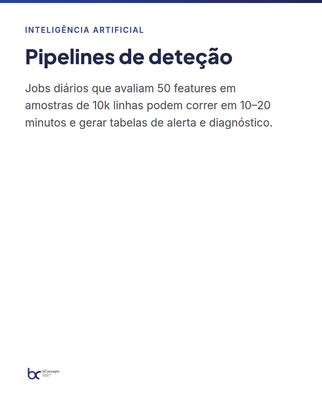
Use Notebooks to compute statistical metrics in rolling windows (e.g., last 7, 30, 90 days) and persist the results. Configure scheduled jobs/pipelines that run KS, PSI tests and analyze SHAP values for production samples. Concretely: a daily pipeline that evaluates 50 critical features on 10k‑row samples can run in 10–20 minutes on a small Data Engineering cluster, generating alert tables and a diagnostic record per alarm.
Finally, expose these results in a Power BI dashboard where analysts can validate alerts and explore drift with drill‑down to the original record. In Power BI, combine trend charts (7/30/90 days), PSI heatmaps per feature and reports with the 100 most atypical examples identified by Mahalanobis distance or outlier scores. This context reduces manual investigation: in a typical session, an analyst can identify the likely cause in 20–40 minutes instead of several hours.
Alerts and automatic triage: from signal to context
An alert without context is noise. When a KS test or a PSI fires, combine multiple signals before issuing a high‑priority alert: anomaly in several correlated features, change in data volume and shifts in SHAP importances increase confidence in the event. Configure severity levels — warning, attention and critical — with distinct thresholds for each level.
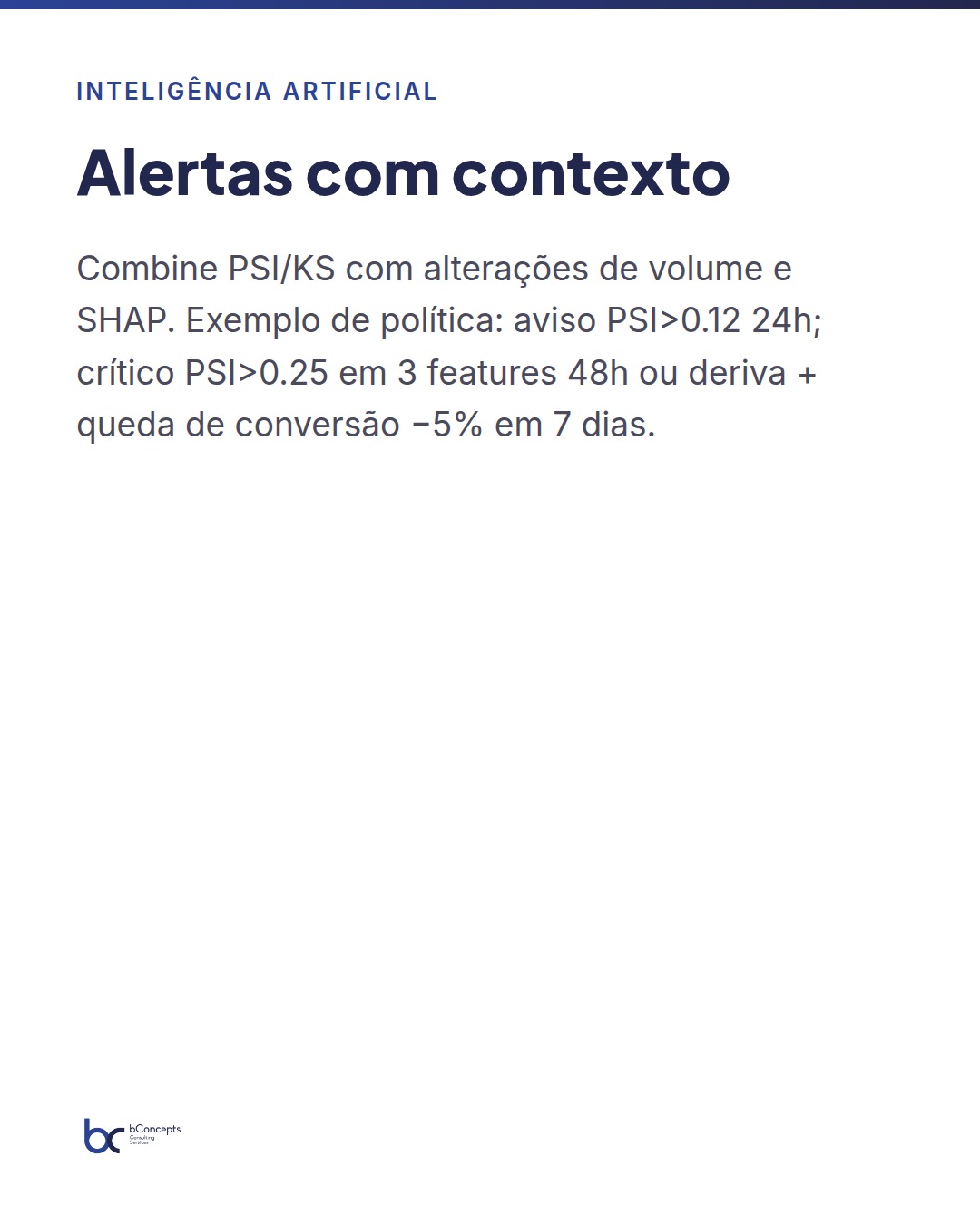
For example, a practical policy: issue a warning when PSI>0.12 for 24 hours in any feature; attention when PSI>0.18 or KS p‑value < 0.01 in two or more features; critical when PSI>0.25 in three critical features for 48 hours or when there is a combination of drift and decline in business metrics (e.g., conversion rate −5% in 7 days). These rules can be encoded in Fabric Pipelines to automate triage actions.
In Fabric, pipelines can trigger automatic actions: send notifications to a Teams channel, create a record in an incident file in the Lakehouse or start another triage pipeline that runs diagnostics (histograms, outlier examples, profile comparisons by segment). This step reduces reaction times: instead of an analyst discovering the problem days later, the team receives rich context for immediate decision. In organizations with strict SLAs, an automated response can reduce detection latency to under 6 hours and accelerate the decision to retrain or mitigate.
Triggering responses: retraining, feature engineering and canary testing
Not all drift requires retraining. Common responses are: 1) adjust transformations (e.g., outlier removal, re‑binning), 2) reweight features or 3) retrain the model with recent data. Define clear policies: automatic retraining thresholds (e.g., PSI>0.25 in three critical features for 48 hours) and manual policies for analytical interventions.
Before retraining in production, run diagnostics: quantify impact on business metrics in historical data, assess availability of recent labels and check whether drift is localized to a segment. For example, if drift occurs only in 10% of traffic (region or new channel), a preferable solution might be model splitting by segment rather than global retraining.
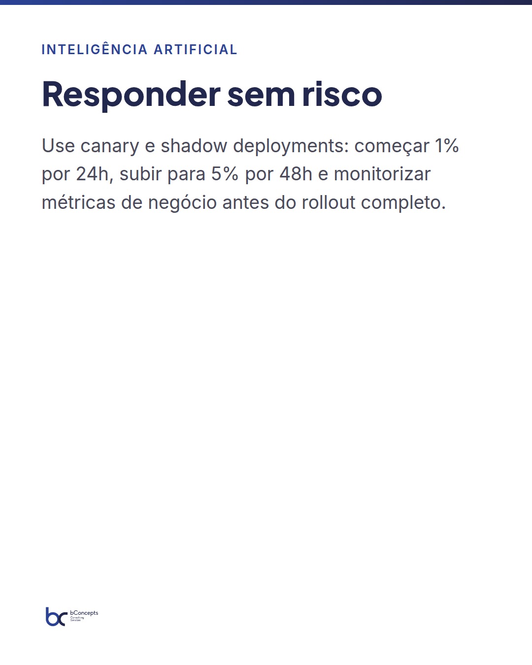
Implement canary and shadow deployments to mitigate risk. A canary exposes a small percentage of traffic to the new model, allowing measurement of business metric deltas before full rollout. In parallel, shadow mode lets you apply the new model offline on real traffic to compare predictions without impacting users. In Fabric, this logic is orchestrated with Pipelines and Notebooks that produce comparative reports and flag regressions with business metrics (e.g., conversion rate, false positive rate). A common practice is to start with a 1% canary for 24 hours, increase to 5% for 48 hours, and only then proceed to 20%+ if there is no regression — throughout this process, monitor p‑values of differences and key business metrics.
Mini practical case: online retail with 80 employees
In an online retail company with 80 employees and an average volume of 10,000 daily sessions, the product team relied on a recommendation model that fed the homepage. The model was retrained biweekly, but over the last three months revenue per visitor fell 6% with no obvious explanation.
We implemented a pipeline in Microsoft Fabric that aggregated features in real time into the Lakehouse, computed PSI and KS in 7/30 day windows, and exposed a Power BI dashboard. Daily instrumentation included summaries per session and per user cohort (new vs returning). Results: the PSI of the feature "time since last purchase" rose to 0.28 and the SHAP importance of this feature decreased 40% compared to training. The system triggered a critical alert. By applying shadow scoring and a 5% traffic canary, we observed an 8% drop in click‑through rate when the old model was used without reweighting.
The operational response was threefold: (1) retraining with adjusted data windows (last 30 days with higher weight), (2) feature reengineering by splitting it into seasonal categories (e.g., 0–7 days, 8–30, >30 with seasonal flags) and (3) implementation of a progressive canary that raised coverage to 50% in five days. Retraining added 3 new context features (active promotions, traffic source, device) that reduced prediction error by 6% (MSE) on validation.
The outcome: recovery of 3.5% revenue per visitor in four weeks and a 40% reduction in false alerts thanks to calibrated thresholds. Operationally, the average investigation time fell from 18 hours to 4 hours and the operating cost associated with monitoring decreased because only 12 of the 200 features were evaluated with full tests daily — the rest were handled by summaries and conditional triggers, saving cluster resources by about 70%.
Detecting drift without context is like looking for a needle in a haystack; integrating telemetry, tests and business makes detection useful.
Best practices for thresholds, windows and costs
Setting thresholds is both scientific and political. Start with conservative rules (PSI>0.1 for observation, >0.2 for investigation) and then calibrate using historical data — what was the impact on commercial metrics when PSI reached 0.18 in the past? Use combined rolling windows: short term (7 days) for rapid detection and medium term (30–90 days) to separate seasonal noise from sustained changes.
Consider computing costs in Fabric: running KS tests on all features daily can be expensive. Strategy: measure summaries (counts, percentiles) in real time and run full tests only when summaries exceed thresholds. For example, instead of running KS for 200 features every day, run daily summaries for the 200 features and KS only for the 20 with percentile changes greater than 10% — this typically reduces costs by 60–80% without material loss of sensitivity.
Additionally, aggregate features by critical segment (e.g., top 20% of users by revenue) to prioritize resources where commercial risk is highest. Document and version threshold policies in the code repository and record the results of each action (alert, investigation, resolution) to learn from history and refine them with real data.
In summary
- Instrument features and metadata in the Lakehouse and compute metrics (PSI, KS, SHAP) in rolling windows.
- Combine statistical signals with operational telemetry before raising high‑priority alerts.
- Implement automatic responses: triage pipelines, shadow scoring and canary deployments to validate interventions.
- Calibrate thresholds with history and prioritize execution resources for critical features and high‑value segments.
Detecting and managing feature drift in Microsoft Fabric is not just a technical initiative — it is a process that requires integration between data, models and business decisions. By centralizing telemetry in the Lakehouse, instrumenting pipelines and operationalizing responses (automatic triage, retraining and canary tests), small and medium organizations can reduce risk and recover value quickly. A phased implementation, starting with 5–10 critical features and scaling with maturity, avoids unnecessary costs and produces quick wins.
Practical next steps: map the critical features of your models, implement distribution summaries in the Lakehouse and develop a notebook that computes PSI/KS daily. Then, define 2–3 thresholds and a response playbook for the first alert. Would you like us to share a notebook template and a Power BI dashboard to get started in 48 hours?